• PowerPoint presentation: 153 KB
• Resources for environmental impacts and Life Cycle Assessment (LCA)

This page is based heavily on the work of Adisa Azapagic et al
as presented in the Appendix of Polymers, the Environment and Sustainable Development [1]
and Box A3 of the Appendix of Sustainable Development in Practice - Case Studies for Engineers and Scientists [2].

Azapagic et al use a problem-oriented approach to the definition of environmental impacts within the Inventory Analysis phase of Life Cycle Assessment under eight categories.  The categories can be directly mapped to both ISO/TR 14047:2003(E) [3], the British Standard BS8905:2011 [4] and the European Environment Agency environmental impacts [5]:

NB: EICF for cork extraction and granulate processing are summarised on a separate page and are not included in the data below.

Non-Renewable/Abiotic Resource Depletion (NRADP) includes depletion of fossil fuels, metals and minerals.  The total impact can be calculated using:

where B_j is the quantity (burden) of the resource used per functional unit (e.g. per kg of product for a chemical) and ec_1,j represents the estimated total world reserves of that resource.  Classification factors for NRADP are given in Table 1.

Global Warming is caused by the atmosphere's ability to reflect some of the heat radiated from the earth's surface. This reflectivity is increased by the greenhouse gases (GHG) in the atmosphere.  Increased emission of GHGs (CO₂, N₂O, CH₄ and volatile organic compounds (VOCs)) will change the heat balance of the earth and result in a warmer climate over future decades.  Global Warming Potential (GWP) is derived by summing the emissions of the GHG multiplied by their respective GWP factors, ec_2,j.  The GWP value is calculated in kg using:

where B_j represents the emission of greenhouse gas j.  GWP factors, ec_2,j, for different greenhouse gases are expressed relative to the GWP of CO₂, which is therefore defined as unity.  The values of the GWP depend on the time horizon over which the global warming effect is assessed.  GWP factors for shorter times (20 years and 50 years) provide an indication of the short-term effects of greenhouse gases on the climate, while GWP values for longer periods (100 years and 500 years) are used to predict the cumulative effects of these gases on the global climate.  Methane is removed from the atmosphere much more rapidly than CO₂ so its short term effect is even greater than is suggested by the 100 year GWP [5].    The classification factors for GWP are given in Table 2a.

The InterGovernmental Panel on Climate Change (IPCC) publication "Climate Change 2007: The Physical Science Basis - Summary for Policymakers" reported:

• atmospheric carbon dioxide at 379 ppm (vs 280 ppm pre-industrial value) with an annual (and increasing) growth rate of 1.9 ppm per year,
• atmospheric methane at 1774 ppb (vs 715 ppb), and
• atmospheric nitrous oxide at 319 ppb (vs 270 ppb) in 2005.

The amount of carbon dioxide released during the manufacture of different materials is given in Table 2b [8].  Timber contains stored carbon dioxide^* from the atmosphere, so whilst some carbon dioxide is released during its harvesting and processing, "there is 8.3 kg of carbon dioxide [sic] absorbed during both the growth and milling process of timber", so no net carbon dioxide is produced.  In the context of "renewable/bio-based" materials, note that the manufacture of fertiliser is ranked as the fifth of 123 UK production sectors for carbon intensity at 4.61 (units are percentage point change at £70/tonne carbon) and its use produces both methane and nitrous oxide emissions [6].  Those industries which are more carbon intensive than fertilisers are cement/lime and plaster at 9.00, electricity production and distribution at 16.07, refined petroleum at 23.44 and, finally, gas distribution at 25.36 [6].

There is a Table of embodied energy values at https://ecm-academics.plymouth.ac.uk/jsummerscales/MATS347/MATS347A9 NFETE.htm#energy.

“styrene is not expected to contribute to global warming” [Health Canada, 1993 and Kuhn et al, 2000]

• Health Canada, Environmental and Workplace Health: Styrene – PSL1, ISBN 0-662-21062-X (1993)
• D Kuhn, MA Kholiq, E Heinzle, B Bühler and A Schmid, Intensification and economic and ecological assessment of a biocatalytic oxyfunctionalization process, Green Chemistry, 2010, 12, 815-827 with supplementary information.

The British Standard PAS 2050:2008 - Specification for the assessment of the life cycle greenhouse gas emissions of goods and services enables a consistent approach to measuring the embodied greenhouse gas emissions from products and services across their lifecycle, and is applicable to a wide range of sectors and product categories.  It is expected that it will form the basis for an internationally agreed standard in this area.

Further reading: H Goosse, PY Barriat, W Lefebvre, MF Loutre and V Zunz, Introduction to climate dynamics and climate modeling, Online textbook, Université Catholique de Louvain, 2008.

Software: CCaLC is a carbon fooprinting tool for estimation of the life cycle greenhouse gas emissions throughout the whole supply chain.  It uses the internationally accepted life cycle methodology defined by ISO 14044 and PAS2050, is claimed to be simple to use by non-experts and comes with comprehensive databases(including the Ecoinvent database).

Acidification is a consequence of acids (and other compounds which can be transformed into acids) being emitted to the atmosphere and subsequently deposited in  surface soils and water.  Increased acidity of these environments can result in negative consequences for coniferous trees (forest dieback) and the death of fish in addition to increased corrosion of manmade structures (buildings, vehicles etc.).  The Vancouver Sun [12] has reported that anthropogenic CO₂ emissions absorbed by the ocean may have pushed local waters through an acidity “tipping point” beyond which shellfish cannot survive: ten million dead scallops are the latest victims in the waters near Qualicum Beach.

Acidification Potential (AP) is based on the contributions of SO₂, NO_x, HCl, NH₃ and HF to the potential acid deposition in the form of H⁺ (protons).  The AP value is calculated in kg using:

where ec_4,j represents the AP of gas j expressed relative to the value for SO₂ and B_j is its emission in kg per functional unit.  Classification factors for AP are given in Table 3.

Nutrient enrichment results from substances (primarily nitrogen and phosphorous from fertilisers) entering ecosystems and disturbing the normal biological balance.  Some organisms may gain an unnatural advantage at the expense of other life forms.  The principal consequence of nutrient enrichment is oxygen depletion, but normally low-nutrient habitats such as moorland can be damaged by such nutrient enrichment.  The use of commercial inorganic fertilisers, in conjunction with increased livestock densities and the concentration of livestock production, has brought about a significant increase in the nutrient load on cultivated land.  This material overload can result in runoff to watercourses leading in turn to eutrophication or contaminated water supply systems [5].  It has been known for decades that high levels of nitrogen deposition have the potential to change plant community composition and biodiversity. However, Emmett [13] has predicted substantial effects from lower, chronic levels of deposition.

Eutrophication Potential (EP) is defined as the potential of nutrients to cause over-fertilisation of water and soil which in turn can result in increased growth of biomass.  The EP value is calculated in kg using:

where B_j is an emission of a species such as N, NO_x, NH₄⁺, PO₄^3-, P and chemical oxygen demand (COD).  The parameters ec_5,j are measured relative to PO₄^3-.  Classification factors for EP are given in Table 4.

Sundqvist [14] references eutrophicating substances to Chemical Oxygen Demand (DOD) with 1 kg of NO₃^- equal to 4.4 kg COD, 1 kg of NO_x equal to 6 kg of COD, 1 kg of NH₃ equal to 16 kg COD and 1 kg phosphorus equal to 140 kg COD.

Kurtz et al [15] found that the survival of larvae in six Lepidoptera species decreased by at least one-third, without clear differences between sorrel- and grass-feeding species, when nitrogen fertiliser was applied to the host plants at rates typically used in current farming practice.

Photochemical Oxidant Formation results from the degradation of the oxides of nitrogen (NO_x) and volatile organic compounds (VOCs) in the presence of light.  Excess ozone can lead to damaged plant leaf surfaces, discolouration, reduced photosynthetic function and ultimately death of the leaf and finally the whole plant.  In animals, it can lead to severe respiratory problems and eye irritation.  Photochemical Oxidants Creation Potential (POCP) is related to the potential for VOCs and oxides of nitrogen to generate photochemical or summer smog.  It is usually expressed relative to the POCP classification factor for ethylene.  The POCP value is calculated in kg using:

where B_j is the emission of the species participating in the formation of summer smog and ec_6,j is the classification factor for photochemical oxidation formation.  Classification factors for ATP are given in Table 5:

Ozone is formed and depleted naturally in the earth's stratosphere (between 15-40 km above the earth's surface).  Halocarbon compounds are persistent synthetic halogen containing organic molecules that can reach the stratosphere leading to more rapid depletion of the ozone.  As the ozone in the stratosphere is reduced more of the ultraviolet rays in sunlight can reach the earth's surface where they can cause skin cancer and reduced crop yields.  Ozone Depletion Potential (ODP) indicates the potential for emissions of chlorofluorocarbon (CFC) compounds and other halogenated hydrocarbons to deplete the ozone layer.  Chlorofluorocarbons are now of minor importance since they were banned by the Montreal Protocol [17].

Fertiliser-induced N₂O emissions are now the single most important driver of stratospheric ozone depletion on a global scale [18].  Extensive farming may now be seeing decreasing yields, and combined with competition for land use between food, fuel and bio-based feedstocks, there is a need for a thorough evaluation of bio-based materials at local, regional, national and global scales [17, 19, 20].  The ODP value is calculated in kg using:

where B_j is the emission of an ozone-depleting gas j.  The ODP factors ec_3,jare expressed relative to the ODP of trichlorofluoromethane (CFC-11) [21].  Classification factors for ODP are given in Table 6.

Human and Eco-Toxicity result from persistent chemicals reaching undesirable concentrations in each of the three elements of the environment (air, soil and water) leading to damage to humans, animals and eco-systems.  The modelling of toxicity in LCA is complicated by the complex chemicals involved and their potential interactions. Azapagic [1, 2] states that “Toxicity estimations in LCA are notoriously unreliable and difficult to quantify”.

While natural products are often assumed to be benign, inhalation of lignocellulosic dust from processing of plant fibres in an inadequately ventilated working environment can lead to narrowing of the airways (byssinosis).

Human Toxicity Potential (HTP) takes account of releases of materials toxic to humans in three distinct media - air (A), water (W) and soil (S).  The HTP value is calculated in kg using:

where ec_7,jA, ec_7,jW and ec_7,jS are human toxicological classification factors for substances emitted to air, water and soil respectively and B_jA, B_jW and B_jS represent the respective emissions of the different toxins to each of the media.  The toxicological factors are calculated using scientific estimates for the acceptable daily intake or tolerable daily intake of the toxic substances.  The human toxicological factors are still at an early stage of development so that HTP can only be taken as an indication and not as an absolute measure of the toxicity potential.  Classification factors for HTP are given in Table 7.

Styrene has an odour threshold 0.08 ppm (parts per million) [22] to 0.32 ppm [23].  Permitted levels in the workplace range from 10 ppm (new build facilities in Sweden) to 100 ppm (e.g. UK) for time weighted average exposure.  The NIOSH (National Institute for Occupational Safety and Health) IDLH (Immediately Dangerous to Life or Health) level for styrene is 700 ppm [24] based on acute inhalation toxicity data in humans [25, 26].

In the United States, the National Toxicology Program 12th Report on Carcinogens [American Composites Manufacturers Association - Regulatory Bulletin - 23 July 2008] has recommended that styrene be listed as "reasonably anticipated to be a human carcinogen".

Aquatic Toxicity Potential (ATP) has a value calculated in m³ using:

where ec_8,jA represents the toxicity classification factors of different aquatic toxic substances and B_jA is their respective emissions to the aquatic ecosystem.  ATP is based on the maximum tolerable concentrations of different toxic substances in water by aquatic organisms.  As with HTP, the classification factors for ATP are still developing and hence should only be used as indicators of potential toxicity.  Classification factors for ATP are given in Table 8.

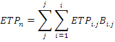
Azapagic [27] has recently stated that "Toxicity estimations in LCA are notoriously unreliable and difficult". While the dilution volume method above does represent an approach previously used , an updated methodology has now been developed (driven by CML in the Netherlands). The method now predominantly used to calculate eco-toxicity (including aquatic ecotoxicity) is based on 1,4-dichlorobenzene equivalence (with units of kg 1,4-DB eq.). Eco-toxicity potential (ETP) is calculated for all three environmental media and comprises five ETP_n indicators:

where n (in the range 1-5) represents freshwater aquatic toxicity, marine aquatic toxicity, freshwater sediment toxicity, marine sediment toxicity and terrestrial ecotoxicity respectively.  ETP_i,j represents the ecotoxicity classification factor for toxic substance j in the compartment i (air, water, soil) and B_i,j is the emission of substance j to compartment i.  ETP is based on the maximum tolerable concentrations of different toxic substances in the environment by different organisms.

References

1. A Azapagic, A Emsley and I Hamerton, Polymers, the Environment and Sustainable Development, John Wiley & Sons, March 2003, ISBN 0-471-87741-7. PU CSH Library.
2. A Azapagic and S Perdan (editors), Sustainable Development in Practice - Case Studies for Engineers and Scientists, Wiley, 2011. ISBN 978-0-470-71872-8. [First edition: John Wiley & Sons, May 2004. ISBN 0-470-85609-2].
3. Environmental management — Life cycle assessment — Illustrative examples on how to apply ISO 14044 to impact assessment situations, International Standard ISO/TR 14047:2012, June 2012. ISBN 978 0 580 72525 8. [First edition: Environmental Management – Life Cycle Impact Assessment – Examples of Application of ISO14042, International Standard PD ISO/TR 14047:2003(E), 11 December 2003. ISBN 0-580-43112-6].
4. BS 8905:2011  Framework for the assessment of the sustainable use of materials - guidance, BSI Group, London, August 2011, withdrawn 08 December 2023.
5. P Kaźmierczyk (editor) with S Moll, M Skovgaard and P Schepelmann, Sustainable use and management of natural resources, EEA Report No 9/2005. ISBN 92-9167-770-1. ISSN 1725-9177.
6. N Stern, The Economics of Climate Change (Stern Review), Cambridge University Press, Cambridge, 2006. ISBN 0-521-70080-9.  PU CSH Library. Executive Summary.
7. DR Shonnard, Evaluating the Environmental Performance of a Flowsheet, in D Allen and D Shonnard, Green Engineering: Environmentally Conscious Design of Chemical Processes, Prentice Hall, 2002. ISBN 0-13-061908-6.
8. Forests, Timber and the Greenhouse Effect, NSW Department of Primary Industries, 13 May 2004.
9. Life cycle assessment of offshore and onshore sited wind power plants based on Vestas V90-3.0MW turbines, Vestas Wind Systems A/s, Randers (DK), 29 March 2005, accessed 08 February 2007 at 11:37.
10. PA Ochoa George, AS Gutiérrez, JB Cogollos Martínez and C Vandecasteele, Cleaner production in a small lime factory by means of process control, Journal of Cleaner Production, 18 (2010), pp. 1171–1176.
11. A Sagastume Gutiérrez, J Van Caneghem, JB Cogollos Martínez and C Vandecasteele, Evaluation of the environmental performance of lime production in Cuba, Journal of Cleaner Production, 31 (2012), pp. 126–136.
12. R Shore, Acidic water blamed for BC’s 10-million scallop die-off, The Vancouver Sun, 26 February 2014.
13. B Emmett, Nitrogen a major driver of biodiversity loss, Acid News, June 2008, (2), 13-15.
14. J-O Sundqvist, Chapter 15: Assessment of Organic Waste Treatment, pages 247-263 in Jo Dewulf and Herman van Langenhove (editors), Renewables-Based Technology: Sustainability Assessment, Wiley, Chichester, 2006.  ISBN 978-0-470-02241-2.  PU CSH Library
15. S Kurze, T Heinken and T Fartmann, Nitrogen enrichment in host plants increases the mortality of common Lepidoptera species, Oecologia, December 2018, 188(4), 1227–1237.
16. Styrene: Part 1 – Environment, European Union Risk Assessment Report, European Chemicals Bureau Institute for Health and Consumer Protection Priority List 1 volume 27, European Commission Joint Research Centre report EUR 20541 EN, 2002.
17. M Weiss, J Haufe, M Carus, M Brandão, S Bringezu, B Hermann and MK Patel, A review of the environmental impacts of biobased materials, Journal of Industrial Ecology, April 2012, 16(S1), S169–S181.
18. AR Ravishankara, JS Daniel and RW Portmann, Nitrous oxide (N2O): the dominant ozone-depleting substance emitted in the 21st century, Science, 2 October 2009, 326(5949), 123-125.
19. E Würdinger, U Roth, A Wegener, R Peche, W Rommel, S Kreibe, A Nikolakis, I Rüdenauer, C Pürschel, P Ballarin, T Knebel, J Borken, A Detzel, H Fehrenbach, J Giegrich, S Möhler, A Patyk, GA Reinhardt, R Vogt, D Mühlberger and J Wante,
    Kunststoffe aus nachwachsenden Rohstoffen: Vergleichende Ökobilanz für Loose-fill-Packmittel aus Stärke bzw. Polystyrol, Projektgemeinschaft BIfA / IFEU / Flo-Pak Endbericht (DBU-Az. 04763), March 2002.
20. M Weiss, J Haufe, M Carus, M Brandão, S Bringezu, B Hermann and MK Patel, A review of the environmental impacts of biobased materials, Journal of Industrial Ecology, April 2012, 16911), 5169-5181.
21. Chemical Profile for trichlorofluoromethane (CAS Number 75-69-4), Scorecard - the pollution information site, accessed 08 February 2006.
22. J May, Solvent odor thresholds for the evaluation of solvent odors in the atmosphere, Staub-Reinhalt, 1966, 26(9), 385-389.
23. JE Amoore and E Hautala, Odor as an aid to chemical safety: odor thresholds compared with threshold limit values and volatilities for 214 industrial chemicals in air and water dilution, Journal of Applied Toxicology, 1983, 3(6), 272-290.
24. Styrene IDLH Documentation, Centers for Disease Control and Prevention, 16 August 1996.
25. Styrene monomer, in AIHA Hygienic guide series. American Industrial Hygiene Association, Akron OH, 1959.
26. RRD Stewart, HC Dodd, ED Baretta and AW Schaffer, Human exposure to styrene vapor, Archives of Environmental Health, 1968, 16(.), 656-662.
27. A Azapagic, Private communication, 25 February 2009.